
I’ve always been fascinated by artificial intelligence, writing software that can solve a problem at hand without hard coding all the combination of branches needed to solve it. Writing software that learns how to solve the problem – with a bit of guidance. I have recently started to dig into this area and I’ve written my very own, with a bit of help, neural network in C#.
This blog post series will help me getting a deeper understanding of the subject by writing about what I’ve done and hopefully it will help you in some way as well. I originally planned to start coding right away and explain the theory as I went along, but I soon realized that it would have been too much at once. Therefore, I’ve decided to split this post into a series of posts where the first one (this one) will take up the theory behind a neural network. The second one will then be the actual implementation and the final one (if any) will discuss some performance issues and other reflections. The final goal is that the network can be trained to solve various problems and I’ll demonstrate it by letting the network solve the XOR-function, the sine-function and recognizing handwritten digits.
Before we get started I just want to clarify that I am by no means an expert, rather the contrary – a beginner, in this topic. This blog series might therefore contain errors, both in mathematical formulas and neural network theory. I’ve “learned” the topic by reading a great book – “Make your own neural network” and then follow up reading online and the content here is therefore influenced by it.
What is a neural network?
I will be brief about what a neural network is since you can find heaps of better information about it elsewhere. In short, a neural network is a network of neurons where each neuron receives one or many input signals from other neurons and emits one or many output signals to other neurons. Each signal is distributed via a weight and a neuron only emits an output if the sum of all inputs exceeds a certain threshold, this means that a neuron does not need to emit an output if the combined inputs are too low, i.e. the sensory stimuli is not strong enough. You’ll see how we can model such a network using just high school maths.
Concept of an Artificial neural network
The concept of a neural network might seem daunting and one might think that creating one would require high level maths. I did. It turns out that we will make a simple network using only the four basic operators (plus, minus, multiplication and division), derivatives and Matrix manipulation (addition and multiplication). Let’s get started :).
Layers of neurons
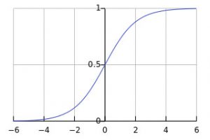
A neural network usually consists of 3 layers – an input, an output and a hidden layer. The hidden layer sits between the input and output layers and can be 0, 1 or many – usually not more than one. The input layer will have equally many neurons, or nodes, as there are inputs. For example, if you have a data-set with 10 properties you will most likely have 10 neurons in your input layer. The output layer will have as many neurons as there are outputs, i.e. for a Boolean output there is one neuron (since a neuron can be ~0 or not) and for recognizing a single digit our output layer will have 10 neurons, one for each digit. The number of neurons in a hidden layer is more of a trial an error kind of value, but a rule of thumb is to have a value in between the number of inputs and outputs.
Neuron Threshold function
As written above, “a neuron only emits an output if the sum of all inputs exceeds a certain threshold“. This function, which is also called the activation function, is responsible for suppressing or emitting the output signal given an input signal. There are many functions used as an activation function, but the one that we will use is the Sigmoid function which has an S-shaped curve with values between 0 and 1. This function will be invoked in each neuron when a signal arrives. Its definition and shape can be seen below.
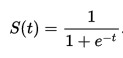
 Sigmoid function*
You will notice that the Sigmoid activation function goes to 0 when X goes to minus infinity and to 1 when X goes towards infinity. The function is only useful for a small X as the output will be between 0 or 1 for X ranging from -4 and from +4. This means that we need to keep our inputs small and expect outputs between 0 and 1. Normally this means that we need to normalize our inputs and then de-normalize our output.
Three layered network with Sigmoid
Signal weights
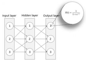
The most central part of a neural network is the weights that are applied to each signal – the network has learned its task when the weights are set to emit the correct output. A weight is applied for each signal as seen in the image below.
Showing signal weights
One usually generates the initial weights randomly between 0 and 1 or -1 and 1. Remember that the Sigmoid activation function will be useful for low X values, i.e. low input signals. If one would have large weights one could easily saturate the network by generating constant on/off signals. Just to drive down the point – if you had a weight of 1000, the input to the Sigmoid function will always be large and the output will always be 1. This is to saturate the network and essentially rendering the neuron redundant.
Let’s give some examples on how to calculate the output for a given neuron. Look at neuron 1 for the hidden layer. Say that O(X) is the output of neuron X and N(1,2) means the first neuron in the second layer. This gives O(N(1,2)) = Sigmoid(O(N(1,1)) * W(1,1) + O(N(2,1)) * W(2,1)). Using the same formula for the second neuron of the hidden layer gives O(N(2,2)) = Sigmoid(O(N(1,1)) * W(1,2) + O(N(2,1)) * W(2,2) + O(N(3,1)) * W(3,2)). I have color coded the sections to make it clearer. So, the output of a given neuron is equal to the Sigmoid of the sum of all inputs where the inputs are weighted. This is done for each neuron in our Neural network!
Output error
We have gone through the formula on how to calculate a neurons output by weighting signals and using an activation function on them. If one would run the network with some inputs and follow these inputs through the network and inspect the final output, i.e. the output from the output layer, one would probably not be satisfied. We would have an error compared to our target value. A network needs to learn a problem to solve it, just pushing inputs and expect a good output without training the network would be very naive. Our objective here is to update our weights so that the output error is low enough (this differs from case to case). When the error is low enough our network will be trained!
Let’s take the Boolean example, i.e. an output value of either true or false. We will then have one output neuron that can emit a value between 0.01 and 0.99 (rounded to 2 decimal points), remember the Sigmoid emits values between 0 and 1. If the target value is 0.99 (true) and our output value is 0.3 then our error is calculated using (target – actual) which equals to 0.69. The dream is an error of 0. Our goal now is to update all the weights in the network so that the error goes towards 0. One such method is Back propagating.
Back propagating errors
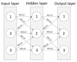
By propagating back, we start with the output layer and work ourselves back towards the input layer, updating our weights along the way. We soon realize that the error of a given neuron is caused by the inputs of many other neurons in the previous layer. Have a look below where the output error is caused by W(2,3) and W(3,3). Therefore, we need to update both W(2,3) and W(3,3) to reduce the error. This is accomplished by updating the error proportionally to their weights – after all, they contributed to the error to the size of their weights. If W(2,3) were twice of W(3,3) then we split the error so that W(2,3) gets twice as much.
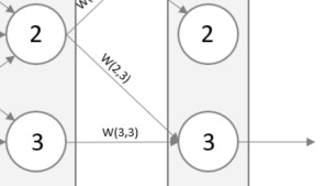
A simple formula can be found for the fraction of the error to use when updating for example W(2,3), that is W(2,3) / W(2,3) + W(3,3). This formula holds true for each layer in the network as we propagate back. While the errors at the output layer is obvious (target – actual) the errors in the hidden neuron is not. This is the reason for the above-mentioned formula. To calculate the error of a hidden neuron one would sum the split errors from all the links connecting forward from the hidden neuron.
Gradient descent
We have learned how to find how much each input signal affected the error but we have not talked about how to find the new weight. How do we find new weights that will reduce the errors (target value – actual value) in the output layer? One way of doing this is using a Brute force approach where, for instance, one would randomly select new weights and inspect the outcome. This guessing game can prove fruitful for very small networks but will quickly become too expensive. Normal networks, with hundreds of neurons per layer, easily has millions of weight combinations which will be very slow to compute.
What if we could find a better way of going towards better weights, it turns out that there is a well-known mathematical method of doing this, a method that will gradually move towards the lowest point – Gradient descent. There probably exists such a function that can calculate the exact weights directly, but such a function would be too complex. Instead, Gradient descent is a good fit since it will allow us to gradually improve our weights by going towards the lowest error given a weight.
In other words, if you imagine a regular coordinate system where the error E is the Y-axis and the weight W is the X-axis, then Gradient descent will move towards the minimum error given a weight. Have a look at the image below, imagine that we are at the dark orange circle and our goal is to be at the brighter orange circle, then Gradient descent can help us find the direction that we need to travel, in this case it is the opposite way of the slope – we need to decrease the weight a bit! You can also see a potential pitfall in this image, if you would decrease the weight by too much, say to 1.25, then you would find yourself moving towards the local minimum at W = 1 which is not the true minimum which is at X = 1.5. We must adjust the weights by a number small enough to prevent overshooting but large enough to have a good performance.
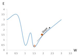
You might think that we can easily find the true minimum using regular algebra and you would be right. However, in neural networks, the output usually depends on more than one value. In the graph above, Y depends on X but in a neural network the output can depend on hundreds of parameters. In fact, the next part of this blog series will demonstrate how to learn to recognize handwritten digits using images of size 28×28 pixels – which is 784 inputs, i.e. the output depends on 784 parameters, try writing that weight adjusting function if you can.
We need to find the slope so that we can move towards the minimum, in other words we need to calculate the derivative dy/dx or in our case dE/dW. The error function is as we seen before (target – actual) and to smooth it a bit we take the square of it. Squaring the value has several benefits, as said, it is a smooth function and as the error moves towards zero the gradient gets smaller which reduces the risk of overshooting. So, the final function for the error is (target – actual)².
So, the error depends on the output and the output depends on the weights (error increases/decreases depending on the output and the output changes as we change the weights), we can then rephrase dE/dW to dE/dO • dO/dW. We have already been over the first bit, which is (target – actual)² and the derivative of that is 2*(target-actual). The second part is more complicated and I won’t go into depth there. We know that the Sigmoid function is applied to the output so the second part, dO/dW, becomes the derivative of the sigmoid function which is already defined and is Sigmoid(x) * (1 – Sigmoid(x)) where x is the weighted sum of all incoming signals. Putting the pieces together gives us a final expression to calculate the adjustment of the weighs, the expression is:
-(target – output) * sigmoid(∑weight*output)*(1-sigmoid(∑weight*output)) * hidden layer output. The constant 2 has been removed since we only want the slope. We have also negated the expression since we want to decrease the weights if the slope is positive and increase the weight if the slope is negative. You will see this function in use in the next post where I’ll implement all this theory into C# code.
Summary
Wow. That was a lot of theory! Let’s sum it up in easy to understand bullets.
- One input layer, zero to many hidden layers and one output layer
- As many neurons in the input layer as there are inputs
- As many neurons in the output layer as there are answers
- Number of neurons in the hidden layer are not pre-defined. A rule of thumb is somewhere in between the number of inputs and outputs.
- Each neuron has an activation function; we are using Sigmoid
- Signal weights are central. Each link between neurons have a weight associated with it.
- The goal is to update the weights so that the network emits the correct output
- Back propagation is used to update the weights from the links based on the errors they contributed to.
- Use Gradient descent to find the lowest error
In the next post, I’ll take this theory and build my very own Neural network, from scratch, in C#!
Do you have any questions, see any errors or just want to get in contact? Do not hesitate to contact me, Andreas Hagsten
Andreas Hagsten
Software Developer, Infozone
* Image source: Wikipedia